Contents
CIRCULAR MOTION OF A RIGID BODY – DISK ROTATION
A rigid body is an object that maintains its shape and volume during motion.
A rigid body can be considered as being made of many small parts marked by points.
Classification of motion based on the movement of individual points of a rigid body:
- Translational
- Rotational
Translational motion
- During the motion, all parts of the rigid body move in the same way and follow the same paths.
- The paths of the points are parallel.
- They travel the same distances in the same time – they have the same velocity.
Rotational motion
Parts of a rigid body move along circular paths, and all those circles lie in planes that are mutually parallel.
The axis of rotation – a straight line that passes through the centers of all circles (can go through the body or outside of it).

Physical quantities describing rotational motion
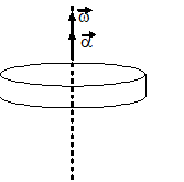
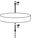
Angular velocity is the physical quantity that describes the speed of rotation of a rigid body.
When a body rotates, its points do not have the same linear velocities – points closer to the axis move slower, while points farther from the axis move faster. However, all points sweep the same angle in the same time, meaning they all have the same angular velocity. That is why angular velocity is used instead of linear velocity.
Angular displacement

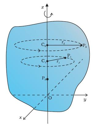
Points 1 and 2 are located at different distances from the axis of rotation. In the same time, they travel different distances and have different displacements.
The radius vectors of points 1 and 2 sweep the same angle in the same time. The angle swept describes the rotational motion. Based on that, angular displacement is defined. Angular displacement is a vector quantity.
Angular acceleration
Disk rotation
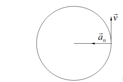
The direction of normal acceleration matches the radius of the circular path, and the vector always points toward the center of the circle. That’s why it’s called radial or centripetal acceleration.
Disk Rotation
1. Objective and Simulation Task
In this lesson, we will create an interactive simulation of a rotating disk. The disk has mass m and radius r.
The two main motion cases we will demonstrate are:
- Uniform Rotation – the disk spins with a constant angular velocity
ω. - Uniformly Accelerated Rotation – the disk starts from rest and accelerates under a constant angular acceleration
α.
The simulation steps include:
- Updating time:
t = t + Δt. - Updating the angular displacement:
Δφ = ω · Δt(for uniform rotation) orΔφ = ω·Δt + (α·Δt²)/2(for uniformly accelerated rotation). - Updating the angle:
φ = φ + Δφ. - Computing the position of point
Mon the disk’s rim in Cartesian coordinates:
x = r · cos(φ)
y = r · sin(φ)
Δt = 0.05 s until the simulation stops.2. Uniform Rotation
When the disk rotates uniformly, the angular velocity ω is constant. At each time step Δt:
- Time update:
t = t + Δt - Position update:
Δφ = ω · Δt, so the new angle isφ = φ + Δφ. - Coordinates of point
Mon the rim:
x = r · cos(φ)
y = r · sin(φ)
At each instant, we draw the position of point M in the 2D plane (on a DrawingPanel) and display a 3D model of the disk that you can rotate with the camera.
This allows students to visually follow how every point on the disk moves in a circular path with the same angular velocity.
3. Uniformly Accelerated Rotation
Now let’s introduce an angular acceleration α. The disk begins from rest (or an initial angular velocity ω0) and accelerates.
Angular acceleration is defined as:
α = dω/dt [rad/s²]
Over the same time interval Δt, the angular displacement Δφ increases because the angular velocity changes:
Δφ = ω·Δt + (α·Δt²)/2ω is the current angular velocity in that step, and after this step it updates as
ω = ω + α·Δt.
- Time update:
t = t + Δt - Angle update:
φ = φ + ω·Δt + (α·Δt²)/2 - Angular velocity update:
ω = ω + α·Δt - Coordinates of point
M:x = r · cos(φ) y = r · sin(φ)
Notice the analogy with linear motion:
s = s0 + v0·t + (a·t²)/2s with φ, v0 with ω, and a with α.
4. Torque and Moment of Inertia
For the disk to accelerate, an external force must act. However, the disk experiences a distribution of forces, not just at a single point. What matters is the torque
produced by the tangential component Ft. For point M at distance r from the rotation axis, the torque is:
τ = Ft · r [N·m]
The normal component Fn passes through the rotation axis, so its torque is zero. Therefore, only the tangential force contributes to rotation.
The measure of inertia in circular motion is the moment of inertia I. For a solid disk:
I = (m·r²)/2m is the disk’s mass and r is its radius.
Newton’s Second Law for Rotation states:
τ = I · αAlso, the angular momentum of the disk about a fixed axis is:
L = I · ωω is the disk’s angular velocity.
5. Practical Simulation Example in EJS
In the EJS environment, the rotating disk simulation includes:
- 3D view of the disk spinning or accelerating around its vertical axis. The camera can be rotated to view the motion from different angles.
-
2D “Top View” projection on a
PlottingPanelshowing the circular trajectory of pointMin the plane. -
Graph of angular velocity
ωover time on a secondPlottingPanel. -
Graphs of the disk’s kinetic and potential energy versus time on a third
PlottingPanel, illustrating energy transfer from rotational kinetic to potential and back in uniformly accelerated motion.
The user can adjust parameters:
- Disk radius
rand massm. - Initial angular velocity
ω0or angular accelerationα. - Time step
Δtfor the simulation updates.
6. Conclusion
Disk rotation is an excellent example for understanding dynamic laws in rotational motion. Through the EJS simulation, you can explore:
- How angular acceleration changes when you increase or decrease the torque
τ. - How the moment of inertia
Iof the disk depends on mass and radius (I = m·r²/2). - How energy transfers between rotational kinetic energy and potential energy (if the disk were lifted).
- How the analogy with linear motion helps calculate the angle
φand angular velocityωover time.
Studying disk rotation via an interactive simulation not only makes learning dynamics laws engaging, but also provides a deep understanding of how torques and moments affect real-world objects in everyday life and engineering applications.