2D Top View and 3D Perspective
The simulation renders both a bird’s-eye view (showing the disc’s outline and rotation) and a 3D view (providing depth).
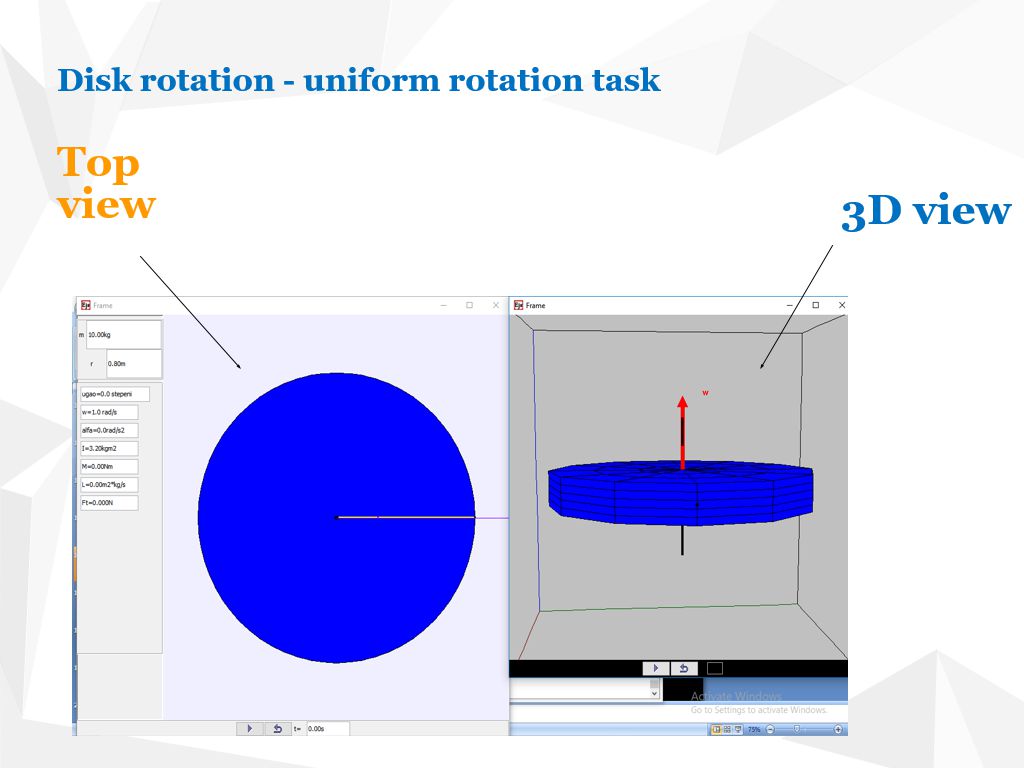
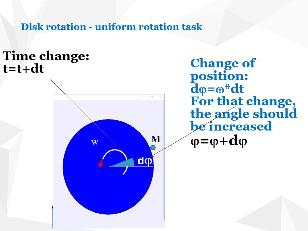
We present a two-view simulation (2D “top” view and 3D perspective) of a uniformly rotating disc. Each step shows how we track a point on the rim and convert between polar and Cartesian coordinates.
The simulation renders both a bird’s-eye view (showing the disc’s outline and rotation) and a 3D view (providing depth).
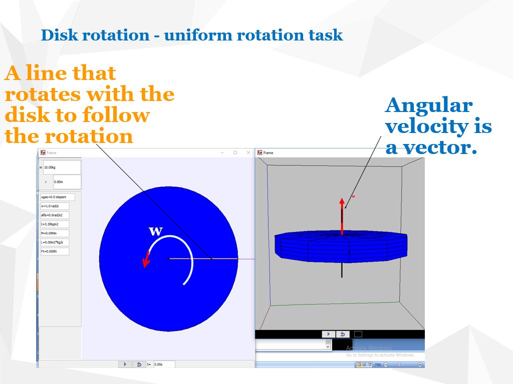
We attach a radial line to point M on the rim. Its instantaneous velocity vector ω·r is shown tangentially.
Let time advance in uniform increments dt (e.g. 0.05 s). The angular displacement per step is dφ = ω·dt.
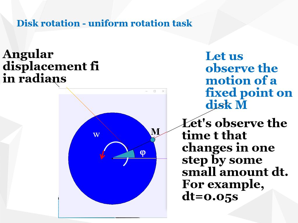
At each iteration:
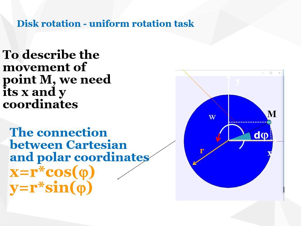
To plot point M in the canvas, convert its polar coordinates (r,φ) into:
x = r·cos(φ) y = r·sin(φ)